16. [Optional] Text: Linear Model Assumptions
Model Assumptions And How To Address Each
Here are the five potential problems related to Multiple Linear Regression that we mentioned in the previous video, that are addressed in Introduction to Statistical Learning:
- Non-linearity of the response-predictor relationships
- Correlation of error terms
- Non-constant Variance and Normally Distributed Errors
- Outliers/ High leverage points
- Multicollinearity
This text is a summary of how to identify whether these problems exist, as well as how to address them.
This is a common interview question asked by statisticians, but its practical importance is hit or miss depending on the purpose of your model. In the upcoming concepts, we will look more closely at specific points that I believe deserve more attention, but below you will see a more exhaustive introduction to each topic. Let's take a closer look at each of these items.
Linearity
The assumption of linearity is that a linear model is the relationship that truly exists between your response and predictor variables. If this isn't true, then your predictions will not be very accurate. Additionally, the linear relationships associated with your coefficients really aren't useful either.
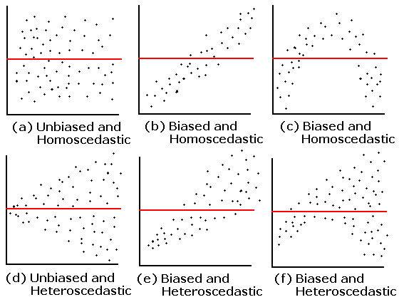
In order to assess if a linear relationship is reasonable, a plot of the residuals (y - \hat{y}) by the predicted values (\hat{y}) is often useful. If there are curvature patterns in this plot, it suggests that a linear model might not actually fit the data, and some other relationship exists between the predictor variables and response. There are many ways to create non-linear models (even using the linear model form), and you will be introduced to a few of these later in this lesson.
In the image at the bottom of this page, these are considered the biased models. Ideally, we want to see a random scatter of points like the top left residual plot in the image.
Correlated Errors
Correlated errors frequently occur when our data are collected over time (like in forecasting stock prices or interest rates in the future) or data are spatially related (like predicting flood or drought regions). We can often improve our predictions by using information from the past data points (for time) or the points nearby (for space).
The main problem with not accounting for correlated errors is that you can often use this correlation to your advantage to better predict future events or events spatially close to one another.
One of the most common ways to identify if you have correlated errors is based on the domain from which the data were collected. If you are unsure, there is a test known as a Durbin-Watson test that is commonly used to assess whether correlation of the errors is an issue. Then ARIMA or ARMA models are commonly implemented to use this correlation to make better predictions.
Non-constant Variance and Normally Distributed Errors
Non-constant variance is when the spread of your predicted values differs depending on which value you are trying to predict. This isn't a huge problem in terms of predicting well. However, it does lead to confidence intervals and p-values that are inaccurate. Confidence intervals for the coefficients will be too wide for areas where the actual values are closer to the predicted values, but too narrow for areas where the actual values are more spread out from the predicted values.
Commonly, a log (or some other transformation of the response variable is done) in order to "get rid" of the non-constant variance. In order to choose the transformation, a Box-Cox is commonly used.
Non-constant variance can be assessed again using a plot of the residuals by the predicted values. In the image at the bottom of the page, non-constant variance is labeled as heteroscedastic. Ideally, we want an unbiased model with homoscedastic residuals (consistent across the range of values).
Though the text does not discuss normality of the residuals, this is an important assumption of regression if you are interested in creating reliable confidence intervals. More on this topic is provided here.
Outliers/Leverage Points
Outliers and leverage points are points that lie far away from the regular trends of your data. These points can have a large influence on your solution. In practice, these points might even be typos. If you are aggregating data from multiple sources, it is possible that some of the data values were carried over incorrectly or aggregated incorrectly.
Other times outliers are accurate and true data points, not necessarily measurement or data entry errors. In these cases, 'fixing' is more subjective. Often the strategy for working with these points is dependent on the goal of your analysis. Linear models using ordinary least squares, in particular, are not very robust. That is, large outliers may greatly change our results. There are techniques to combat this - largely known as regularization techniques. These are beyond the scope of this class, but they are quickly discussed in the free course on machine learning.
Multi-collinearity
Multicollinearity is when we have predictor variables that are correlated with one another. One of the main concerns of multicollinearity is that it can lead to coefficients being flipped from the direction we expect from simple linear regression.
One of the most common ways to identify multicollinearity is with bivariate plots or with variance inflation factors (or VIFs). This is a topic we will dive into in the next concept, so we won't spend as much time on it here.
